Bechdel analysis using the `tidyverse`

This vignette is based on tidyverse-ifying the R code here and reproducing some of the plots and analysis done in the 538 story entitled “The Dollar-And-Cents Case Against Hollywood’s Exclusion of Women” by Walt Hickey available here.

Load required packages to reproduce analysis. Also load the bechdel dataset for analysis.

library(fivethirtyeight)
library(ggplot2)
library(dplyr)
library(knitr)
library(magrittr)
library(broom)
library(stringr)
library(ggthemes)
library(scales)
# Turn off scientific notation
options(scipen = 99)

Filter to only 1990 - 2013

Focus only on films from 1990 to 2013

bechdel90_13 <- bechdel %>% filter(between(year, 1990, 2013))

Calculate variables

Create international gross only and return on investment (ROI) columns and add to bechdel_90_13 data frame

bechdel90_13 %<>% 
  mutate(int_only = intgross_2013 - domgross_2013,
         roi_total = intgross_2013 / budget_2013,
         roi_dom = domgross_2013 / budget_2013,
         roi_int = int_only / budget_2013)

Create `generous` variable

bechdel90_13 %<>%
  mutate(generous = ifelse(test = clean_test %in% c("ok", "dubious"),
                           yes = TRUE,
                           no = FALSE))

Determine median ROI and budget based on categories

ROI_by_binary <- bechdel90_13 %>% 
  group_by(binary) %>% 
  summarize(median_ROI = median(roi_total, na.rm = TRUE))
ROI_by_binary

## # A tibble: 2 × 2
##   binary median_ROI
##   <chr>       <dbl>
## 1 FAIL         2.45
## 2 PASS         2.70

bechdel90_13 %>% 
  summarize(
    `Median Overall Return on Investment` = median(roi_total, na.rm = TRUE))

## # A tibble: 1 × 1
##   `Median Overall Return on Investment`
##                                   <dbl>
## 1                                  2.57

budget_by_binary <- bechdel90_13 %>% 
  group_by(binary) %>% 
  summarize(median_budget = median(budget_2013, na.rm = TRUE))
budget_by_binary

## # A tibble: 2 × 2
##   binary median_budget
##   <chr>          <dbl>
## 1 FAIL       48385984.
## 2 PASS       31070724

bechdel90_13 %>% 
  summarize(`Median Overall Budget` = median(budget_2013, na.rm = TRUE))

## # A tibble: 1 × 1
##   `Median Overall Budget`
##                     <int>
## 1                37878971

View Distributions

Look at the distributions of budget, international gross, ROI, and their logarithms

ggplot(data = bechdel90_13, mapping = aes(x = budget)) +
  geom_histogram(color = "white", bins = 20) +
  labs(title = "Histogram of budget")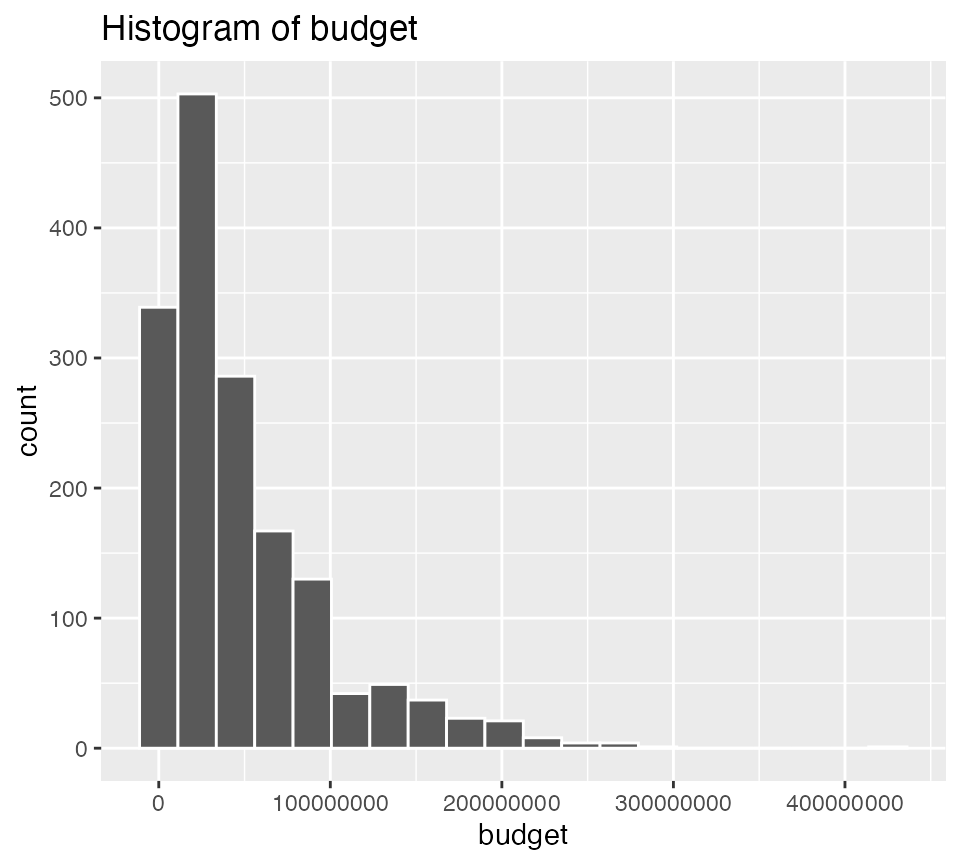

ggplot(data = bechdel90_13, mapping = aes(x = log(budget))) +
  geom_histogram(color = "white", bins = 20) +
  labs(title = "Histogram of Logarithm of Budget")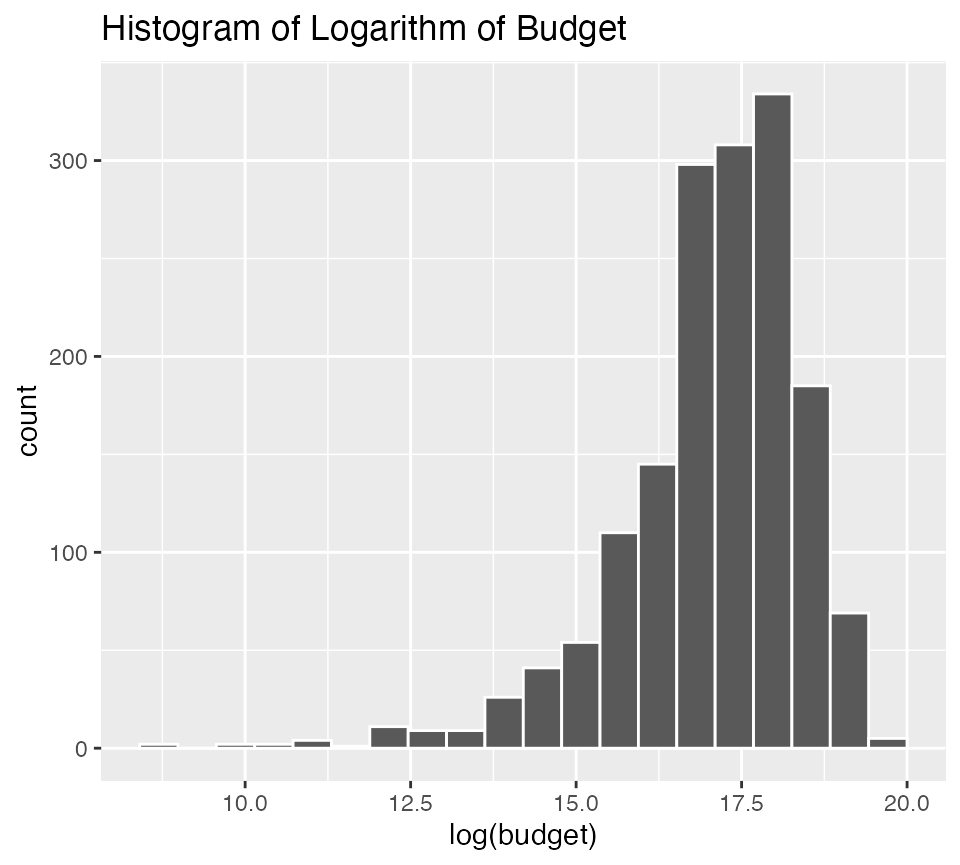

ggplot(data = bechdel90_13, mapping = aes(x = intgross_2013)) +
  geom_histogram(color = "white", bins = 20) +
  labs(title = "Histogram of International Gross")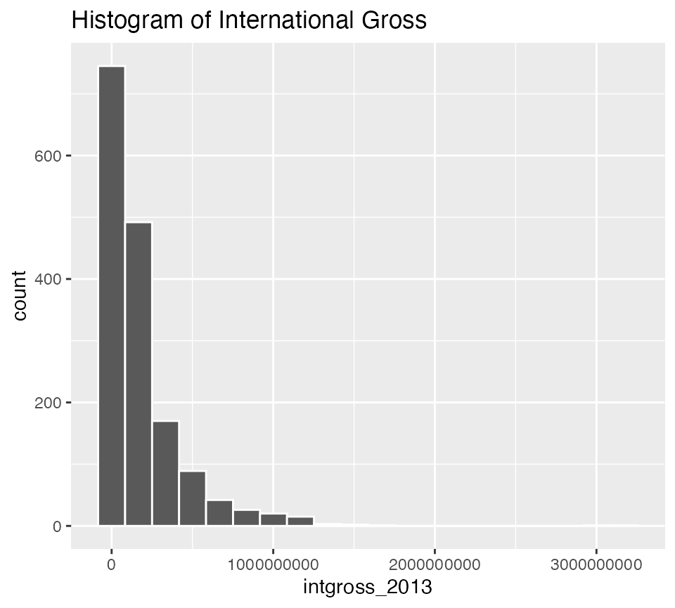

ggplot(data = bechdel90_13, mapping = aes(x = log(intgross_2013))) +
  geom_histogram(color = "white", bins = 20) +
  labs(title = "Histogram of Logarithm of International Gross")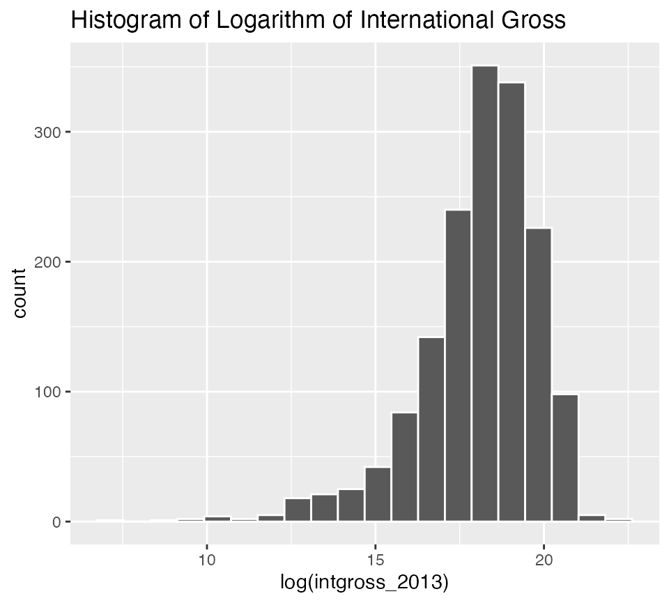

ggplot(data = bechdel90_13, mapping = aes(x = roi_total)) +
  geom_histogram(color = "white", bins = 20) +
  labs(title = "Histogram of ROI")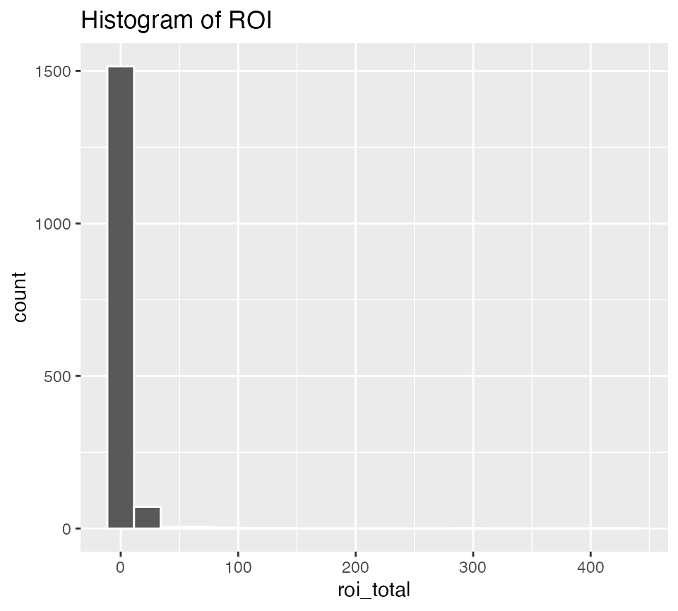

The previous distributions were skewed, but ROI is so skewed that purposefully limiting the x-axis may reveal a bit more information about the distribution: (Suggested by Mustafa Ascha.)

ggplot(data = bechdel90_13, mapping = aes(x = roi_total)) +
  geom_histogram(color = "white", bins = 20) +
  labs(title = "Histogram of ROI") +
  xlim(0, 25)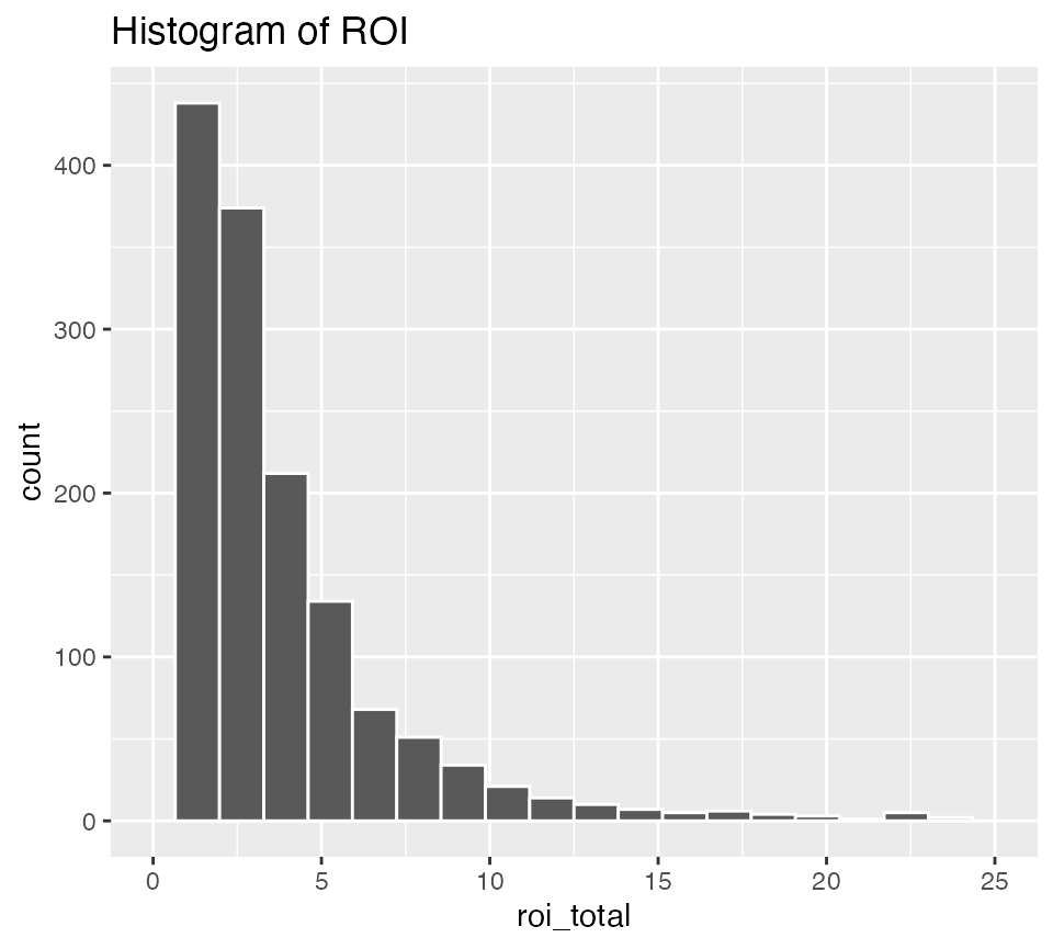

ggplot(data = bechdel90_13, mapping = aes(x = log(roi_total))) +
  geom_histogram(color = "white", bins = 20) +
  labs(title = "Histogram of Logarithm of ROI")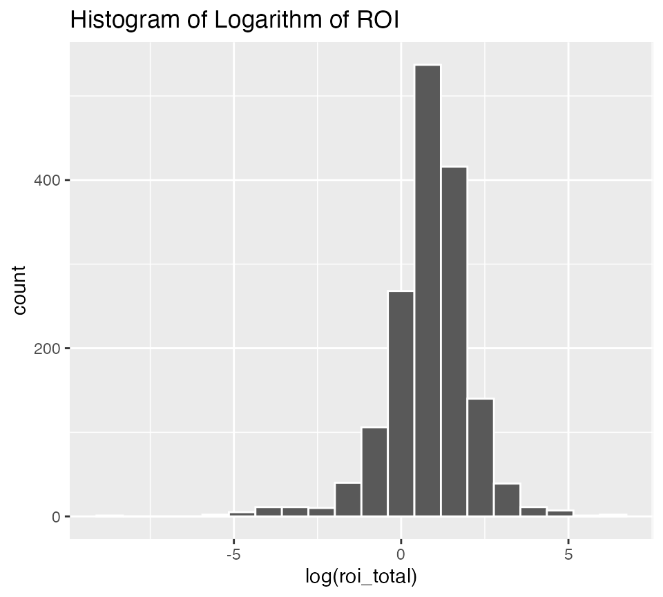

Linear Regression Models

Movies with higher budgets make more international gross revenues using logarithms on both variables

ggplot(data = bechdel90_13, 
       mapping = aes(x = log(budget_2013), y = log(intgross_2013))) +
  geom_point() +
  geom_smooth(method = "lm", se = FALSE)

## `geom_smooth()` using formula 'y ~ x'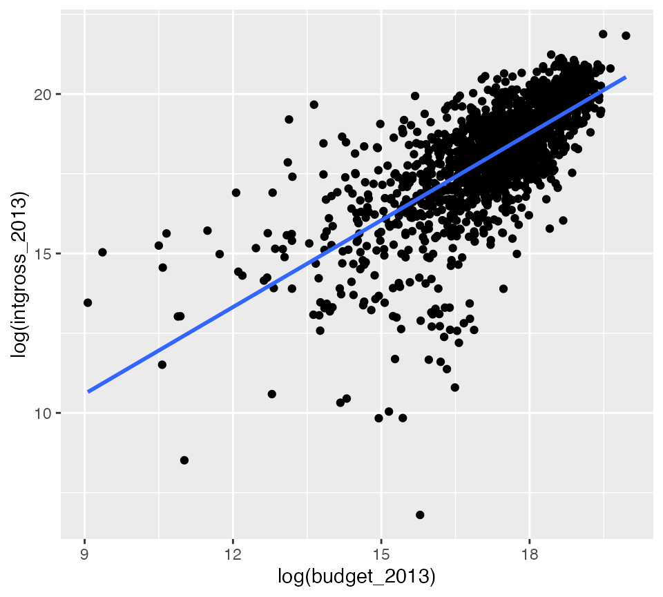

gross_vs_budget <- lm(log(intgross_2013) ~ log(budget_2013), 
                      data = bechdel90_13)
tidy(gross_vs_budget)

## # A tibble: 2 × 5
##   term             estimate std.error statistic   p.value
##   <chr>               <dbl>     <dbl>     <dbl>     <dbl>
## 1 (Intercept)         2.43     0.390       6.23 5.84e- 10
## 2 log(budget_2013)    0.907    0.0225     40.3  1.20e-245

Bechdel dummy is not a significant predictor of `log(intgross_2013)` assuming `log(budget_2013)` is in the model

Note that the regression lines nearly completely overlap.

ggplot(data = bechdel90_13, 
       mapping = aes(x = log(budget_2013), y = log(intgross_2013), 
                     color = binary)) +
  geom_point() +
  geom_smooth(method = "lm", se = FALSE)

## `geom_smooth()` using formula 'y ~ x'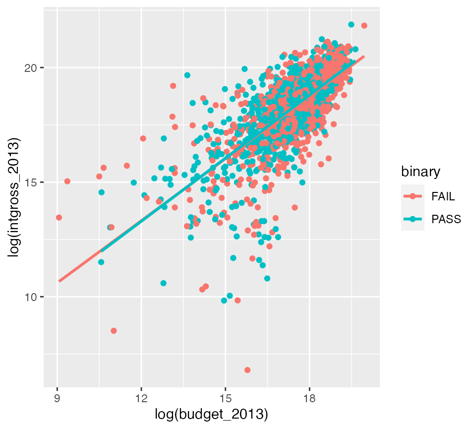

gross_vs_budget_binary <- lm(log(intgross_2013) ~ log(budget_2013) + factor(binary), 
                      data = bechdel90_13)
tidy(gross_vs_budget_binary)

## # A tibble: 3 × 5
##   term               estimate std.error statistic   p.value
##   <chr>                 <dbl>     <dbl>     <dbl>     <dbl>
## 1 (Intercept)          2.36      0.399      5.91  4.10e-  9
## 2 log(budget_2013)     0.910     0.0228    40.0   3.39e-243
## 3 factor(binary)PASS   0.0539    0.0635     0.849 3.96e-  1

Note the \(p\)-value on factor(binary)PASS here that is around 0.40.

Movies with higher budgets have lower ROI

ggplot(data = bechdel90_13, 
       mapping = aes(x = log(budget_2013), y = log(roi_total))) +
  geom_point() +
  geom_smooth(method = "lm", se = FALSE)

## `geom_smooth()` using formula 'y ~ x'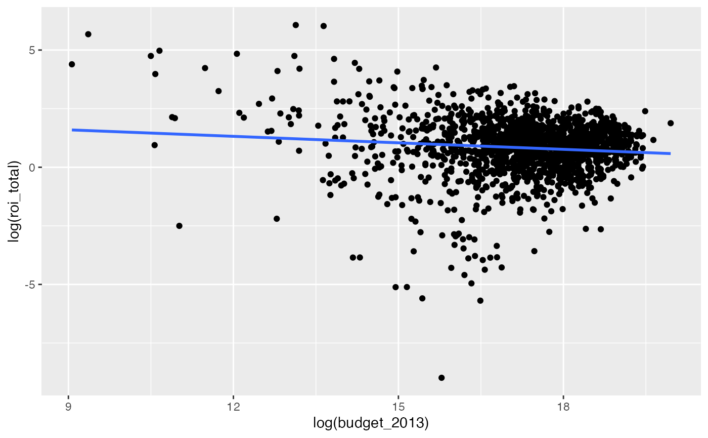

roi_vs_budget <- lm(log(roi_total) ~ log(budget_2013), 
                      data = bechdel90_13)
tidy(roi_vs_budget)

## # A tibble: 2 × 5
##   term             estimate std.error statistic  p.value
##   <chr>               <dbl>     <dbl>     <dbl>    <dbl>
## 1 (Intercept)        2.43      0.390       6.23 5.84e-10
## 2 log(budget_2013)  -0.0926    0.0225     -4.11 4.16e- 5

Note the negative coefficient here on log(budget_2013) and its corresponding small \(p\)-value.

Bechdel dummy is not a significant predictor of `log(roi_total)` assuming `log(budget_2013)` is in the model

Note that the regression lines nearly completely overlap.

ggplot(data = bechdel90_13, 
       mapping = aes(x = log(budget_2013), y = log(roi_total), 
                     color = binary)) +
  geom_point() +
  geom_smooth(method = "lm", se = FALSE)

## `geom_smooth()` using formula 'y ~ x'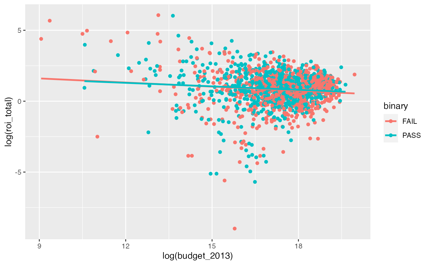

roi_vs_budget_binary <- lm(log(roi_total) ~ log(budget_2013) + factor(binary), 
                      data = bechdel90_13)
tidy(roi_vs_budget_binary)

## # A tibble: 3 × 5
##   term               estimate std.error statistic       p.value
##   <chr>                 <dbl>     <dbl>     <dbl>         <dbl>
## 1 (Intercept)          2.36      0.399      5.91  0.00000000410
## 2 log(budget_2013)    -0.0899    0.0228    -3.95  0.0000810    
## 3 factor(binary)PASS   0.0539    0.0635     0.849 0.396

Note the \(p\)-value on factor(binary)PASS here that is around 0.40.

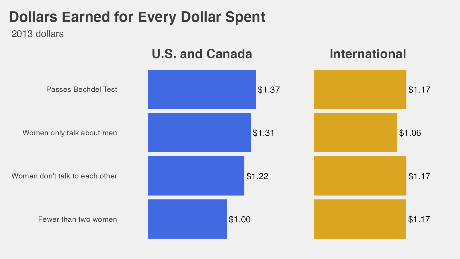
Dollars Earned for Every Dollar Spent graphic

Calculating the values and creating a tidy data frame

passes_bechtel_rom <- bechdel90_13 %>% 
  filter(generous == TRUE) %>% 
  summarize(median_roi = median(roi_dom, na.rm = TRUE))
median_groups_dom <- bechdel90_13 %>% 
  filter(clean_test %in% c("men", "notalk", "nowomen")) %>% 
  group_by(clean_test) %>% 
  summarize(median_roi = median(roi_dom, na.rm = TRUE))
pass_bech_rom <- tibble(clean_test = "pass", 
                  median_roi = passes_bechtel_rom$median_roi)
med_groups_dom_full <- bind_rows(pass_bech_rom, median_groups_dom) %>% 
  mutate(group = "U.S. and Canada")

passes_bechtel_int <- bechdel90_13 %>% 
  filter(generous == TRUE) %>% 
  summarize(median_roi = median(roi_int, na.rm = TRUE))
median_groups_int <- bechdel90_13 %>% 
  filter(clean_test %in% c("men", "notalk", "nowomen")) %>% 
  group_by(clean_test) %>% 
  summarize(median_roi = median(roi_int, na.rm = TRUE))
pass_bech_int <- tibble(clean_test = "pass", 
                  median_roi = passes_bechtel_int$median_roi)
med_groups_int_full <- bind_rows(pass_bech_int, median_groups_int) %>% 
  mutate(group = "International")
med_groups <- bind_rows(med_groups_dom_full, med_groups_int_full) %>% 
  mutate(clean_test = str_replace_all(clean_test, 
                                      "pass",
                                      "Passes Bechdel Test"),
         clean_test = str_replace_all(clean_test, "men",
                                      "Women only talk about men"),
         clean_test = str_replace_all(clean_test, "notalk",
                                      "Women don't talk to each other"),
         clean_test = str_replace_all(clean_test, "nowoWomen only talk about men",
                                      "Fewer than two women"))
med_groups %<>% mutate(clean_test = factor(clean_test, 
                                 levels = c("Fewer than two women", 
                                            "Women don't talk to each other",
                                            "Women only talk about men",
                                            "Passes Bechdel Test"))) %>% 
  mutate(group = factor(group, levels = c("U.S. and Canada", "International"))) %>% 
  mutate(median_roi_dol = dollar(median_roi))

Using only a few functions to plot

ggplot(data = med_groups, mapping = aes(x = clean_test, y = median_roi, 
                                        fill = group)) +
  geom_bar(stat = "identity") +
  facet_wrap(~ group) +
  coord_flip() +
  labs(title = "Dollars Earned for Every Dollar Spent", subtitle = "2013 dollars") +
  scale_fill_fivethirtyeight() +
  theme_fivethirtyeight()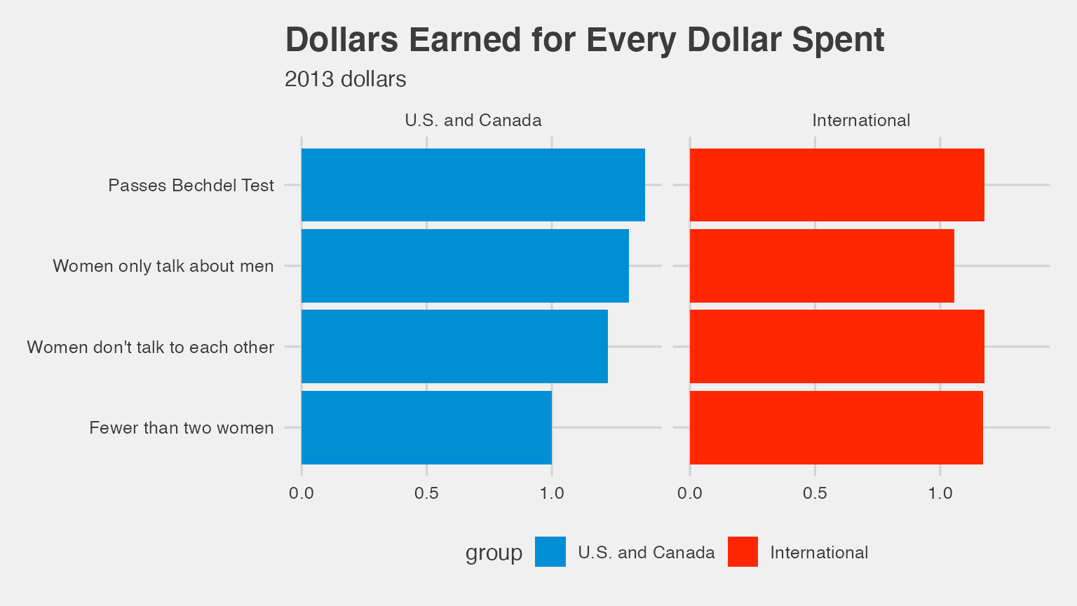

Attempt to fully reproduce Dollars Earned for Every Dollar Spent plot using ggplot

ggplot(data = med_groups, mapping = aes(x = clean_test, y = median_roi, 
                                        fill = group)) +
  geom_bar(stat = "identity") +
  geom_text(aes(label = median_roi_dol), hjust = -0.1) +
  scale_y_continuous(expand = c(.25, 0)) +
  coord_flip() +
  facet_wrap(~ group) +
  scale_fill_manual(values = c("royalblue", "goldenrod")) +
  labs(title = "Dollars Earned for Every Dollar Spent", subtitle = "2013 dollars") +
  theme_fivethirtyeight() +
  theme(plot.title = element_text(hjust = -1.6), 
        plot.subtitle = element_text(hjust = -0.4),
        strip.text.x = element_text(face = "bold", size = 16),
        panel.grid.major = element_blank(), 
        panel.grid.minor = element_blank(),
        axis.title.x = element_blank(),
        axis.text.x = element_blank(),
        axis.ticks.x = element_blank()) +
  guides(fill = FALSE)

## Warning: `guides(<scale> = FALSE)` is deprecated. Please use `guides(<scale> =
## "none")` instead.

Chester Ismay

2021-10-05

Filter to only 1990 - 2013

Calculate variables

Create `generous` variable

Determine median ROI and budget based on categories

View Distributions

Linear Regression Models

Movies with higher budgets make more international gross revenues using logarithms on both variables

Bechdel dummy is not a significant predictor of `log(intgross_2013)` assuming `log(budget_2013)` is in the model

Movies with higher budgets have lower ROI

Bechdel dummy is not a significant predictor of `log(roi_total)` assuming `log(budget_2013)` is in the model

Dollars Earned for Every Dollar Spent graphic

Bechdel analysis using the tidyverse

Chester Ismay

2021-10-05

Filter to only 1990 - 2013

Calculate variables

Create generous variable

Determine median ROI and budget based on categories

View Distributions

Linear Regression Models

Movies with higher budgets make more international gross revenues using logarithms on both variables

Bechdel dummy is not a significant predictor of log(intgross_2013) assuming log(budget_2013) is in the model

Movies with higher budgets have lower ROI

Bechdel dummy is not a significant predictor of log(roi_total) assuming log(budget_2013) is in the model

Dollars Earned for Every Dollar Spent graphic

Bechdel analysis using the `tidyverse`

Create `generous` variable

Bechdel dummy is not a significant predictor of `log(intgross_2013)` assuming `log(budget_2013)` is in the model

Bechdel dummy is not a significant predictor of `log(roi_total)` assuming `log(budget_2013)` is in the model