Gender in Comic Books

This vignette is based on 538 study : Comic Books Are Still Made By Men, For Men And About Men study about Marvel and DC characters since ~1939 until 2014 (August 24th) and aims at investigating the features of Comic Books characters according their gender / Publisher.

#load packages and csv file
library(fivethirtyeight)
library(ggplot2)
library(dplyr)
library(readr)
library(tidyr)
library(lubridate)
library(janitor)
library(knitr)
library(grid)
library(fmsb)
library(wordcloud)
library(gridExtra)

Overview plots

Note as of 2020-07-18: The entire comic_charachters dataset is available in the fivethirtyeightdata package. Instructions to download the fivethirtyeightdata package are given when you load the fivethirtyeight package. Alternately, you can run the following:

install.packages(fivethirtyeightdata,
  repos = "https://fivethirtyeightdata.github.io/drat/",
  type = "source"
)

Load full dataset using code in ?comic_characters help file. Note we need to do this since fivethirtyeight::comic_characters only contains a preview of the first 10 rows of the full dataset.

# Get DC characters:
comic_characters_dc <-
  "https://github.com/fivethirtyeight/data/raw/master/comic-characters/dc-wikia-data.csv" %>%
  read_csv() %>%
  clean_names() %>%
  mutate(publisher = "DC")

# Get Marvel characters:
comic_characters_marvel <-
  "https://github.com/fivethirtyeight/data/raw/master/comic-characters/marvel-wikia-data.csv" %>%
  read_csv() %>%
  clean_names() %>%
  mutate(publisher = "Marvel")

# Merge two dataset and perform further data wrangling:
comic_characters <-
  comic_characters_dc %>%
  bind_rows(comic_characters_marvel) %>%
  separate(first_appearance, c("year2", "month"), ", ", remove = FALSE) %>%
  mutate(
    # If month was missing, set as January and day as 01:
    month = ifelse(is.na(month), "01", month),
    day = "01",
    # Note some years missing:
    date = ymd(paste(year, month, day, sep = "-")),
    align = factor(
      align,
      levels = c("Bad Characters", "Reformed Criminals", "Netural Characters", "Good Characters"),
      ordered = TRUE)
  ) %>%
  select(publisher, everything(), -c(year2, day))

Overview plots

percentage of Gender per publisher.
raw number of characters per publisher.

#calculate raw number and percentage of each gender for each publisher
raw_number_per_publisher <- comic_characters %>%
  group_by(publisher) %>%
  summarise(number = n()) %>%
  arrange(-number)

percent_gen_pub <- comic_characters %>%
  group_by(sex, publisher) %>%
  summarise(number = n()) %>%
  arrange(-number) %>%
  group_by(publisher) %>%
  mutate(countT = sum(number)) %>%
  group_by(sex) %>%
  mutate(
    percentage = (100*number/countT),
    label = paste0(round(percentage, 2)))

#plot percentage of each gender for each publisher
percentage_per_publisher <- ggplot(data = percent_gen_pub,aes(x = sex,y = percentage, fill = publisher)) +
  geom_bar(width = 0.9, stat = "identity", position = 'dodge') +
  theme(axis.text.x = element_text(angle = 45, hjust = 1),legend.position = 'none') +
  geom_text(aes(label = label), position=position_dodge(width = 0.9), vjust = -0.25,size = 2.5) +
  scale_fill_manual(values = c("#3B9AB2","#EBCC2A")) +
  xlab('') +
  ylab('Percentage')

raw_number_per_publisher <- ggplot(data = raw_number_per_publisher, aes(x = publisher, y = number, fill = publisher)) +
  geom_bar(width = 0.1, stat = "identity") +
  coord_flip() +
  scale_fill_manual(values = c("#3B9AB2","#EBCC2A")) +
  xlab('') +
  ylab('') +
  theme(legend.position = 'None')

grid.arrange(percentage_per_publisher, raw_number_per_publisher, ncol=2)

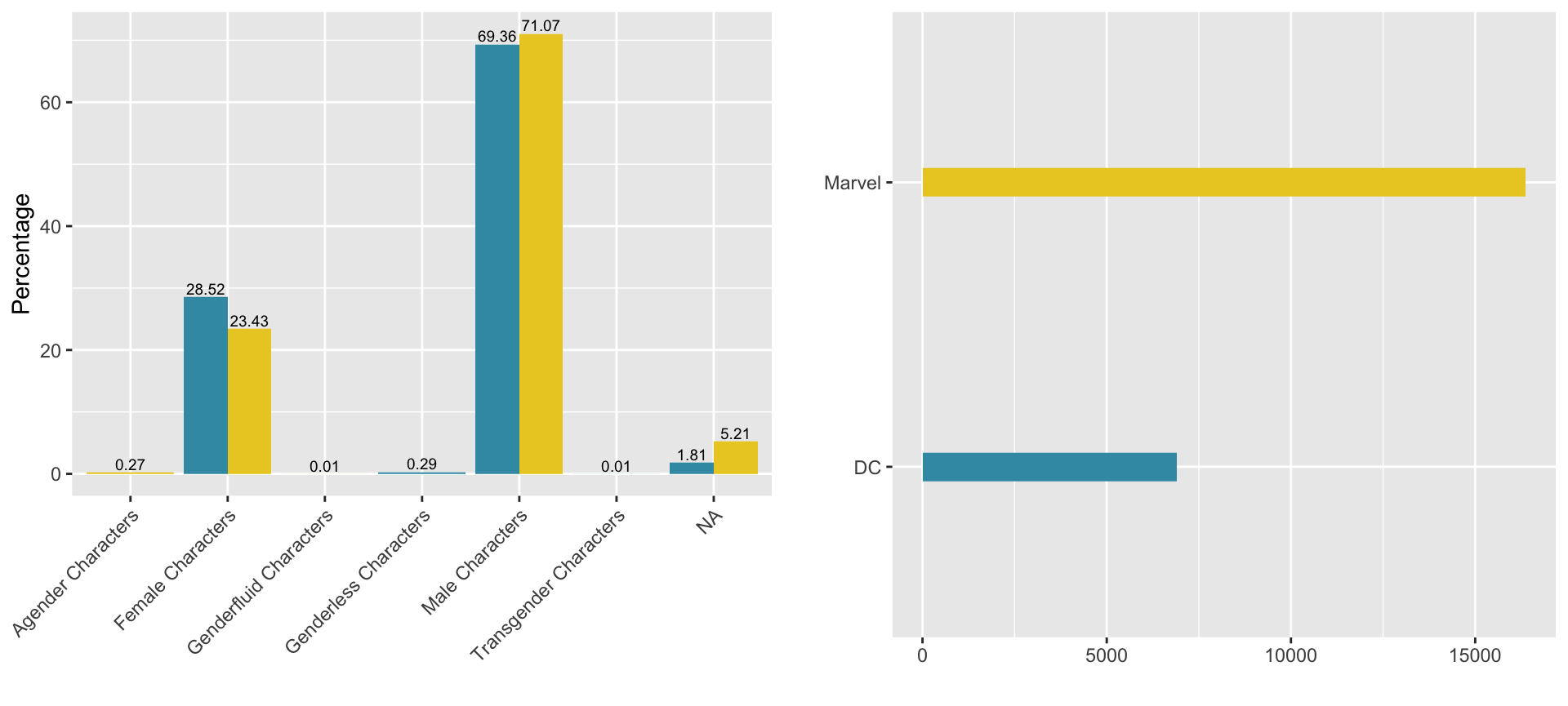
Marvel has more than the double of number of characters compared to DC.
Male are more present in both publishers compared to Female on a ~2.5:1 ratio, while LGBT characters represent less than 1 percent.

Number of Characters vs. Time

#select data with no NA's for sex and date and groupby

#define list of gender per publisher
gender_list_marvel <- c("Female Characters", "Male Characters", "Genderfluid Characters","Agender Characters")
gender_list_dc <- c("Female Characters", "Male Characters", "Genderless Characters","Transgender Characters")

marvel_vs_time <- comic_characters %>%
  filter(publisher == 'Marvel' & !is.na(month) & !is.na(sex)) %>%
  group_by(year, month, sex) %>%
  summarise(number = n()) %>%
  mutate(
    sex_ordered = factor(sex, levels = gender_list_marvel),
    month_ordered = factor(month, levels = month.name))

dc_vs_time <- comic_characters %>%
  filter(publisher == 'DC' & month!= "Holiday" & !is.na(month) & !is.na(sex)) %>%
  mutate(month = ifelse(month=="01","January",month)) %>%
  group_by(year, month, sex) %>% summarise(number = n()) %>%
  mutate(
    sex_ordered = factor(sex, levels = gender_list_dc),
    month_ordered = factor(month, levels = month.name))

plot_marvel_time <- ggplot(data = marvel_vs_time, aes(year, month_ordered)) +
  geom_tile(aes(fill = number),colour = "white") +
  scale_fill_gradient(low = "#EBCC2A", high = "black") +
  facet_wrap(~ sex_ordered, ncol = 4) +
  theme(axis.title.x = element_blank(), axis.ticks.x = element_blank(), axis.title.y = element_blank(), axis.ticks.y =  element_blank(), legend.position = 'right', legend.title = element_blank(), legend.key.size = unit(.2, "cm")) +
  xlim(1935,2015)

plot_dc_time <- ggplot(data = dc_vs_time, aes(year, month_ordered)) + geom_tile(aes(fill = number),colour = "white") +
  scale_fill_gradient(low = "#3B9AB2", high = "black") +
  facet_wrap(~ sex_ordered, ncol = 4) +
  theme(axis.title.x = element_blank() ,axis.ticks.x = element_blank(), axis.title.y = element_blank(), axis.ticks.y = element_blank(), legend.position = 'right', legend.title = element_blank(), legend.key.size = unit(.2, "cm")) +
  xlim(1935,2015)

grid.arrange(rbind(ggplotGrob(plot_marvel_time), ggplotGrob(plot_dc_time), size = "last"))

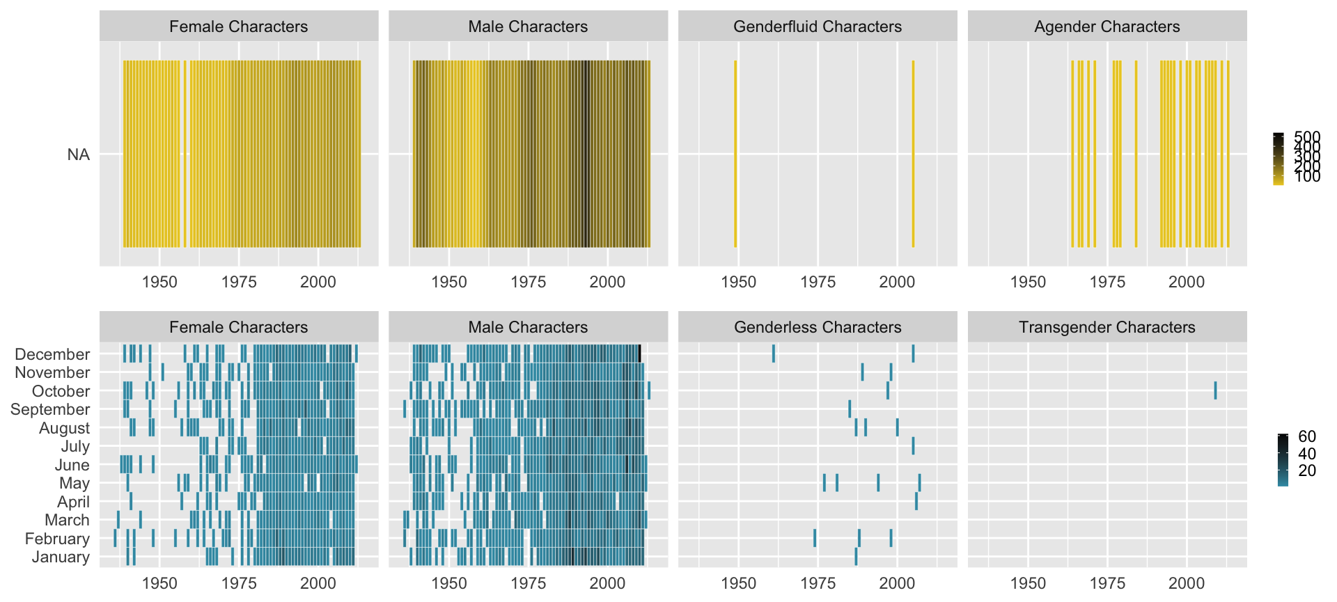
Most of the characters are either Female or Male for both publishers.
There is a gap in character’s creation (for both publishers) ~1955-1960.
The increase in Female characters appear early for Marvel (~1970) while it was in the late 70’s for DC comics.
LGBT characters appear in the late 70’s (DC) and in the late 60’s (Marvel).

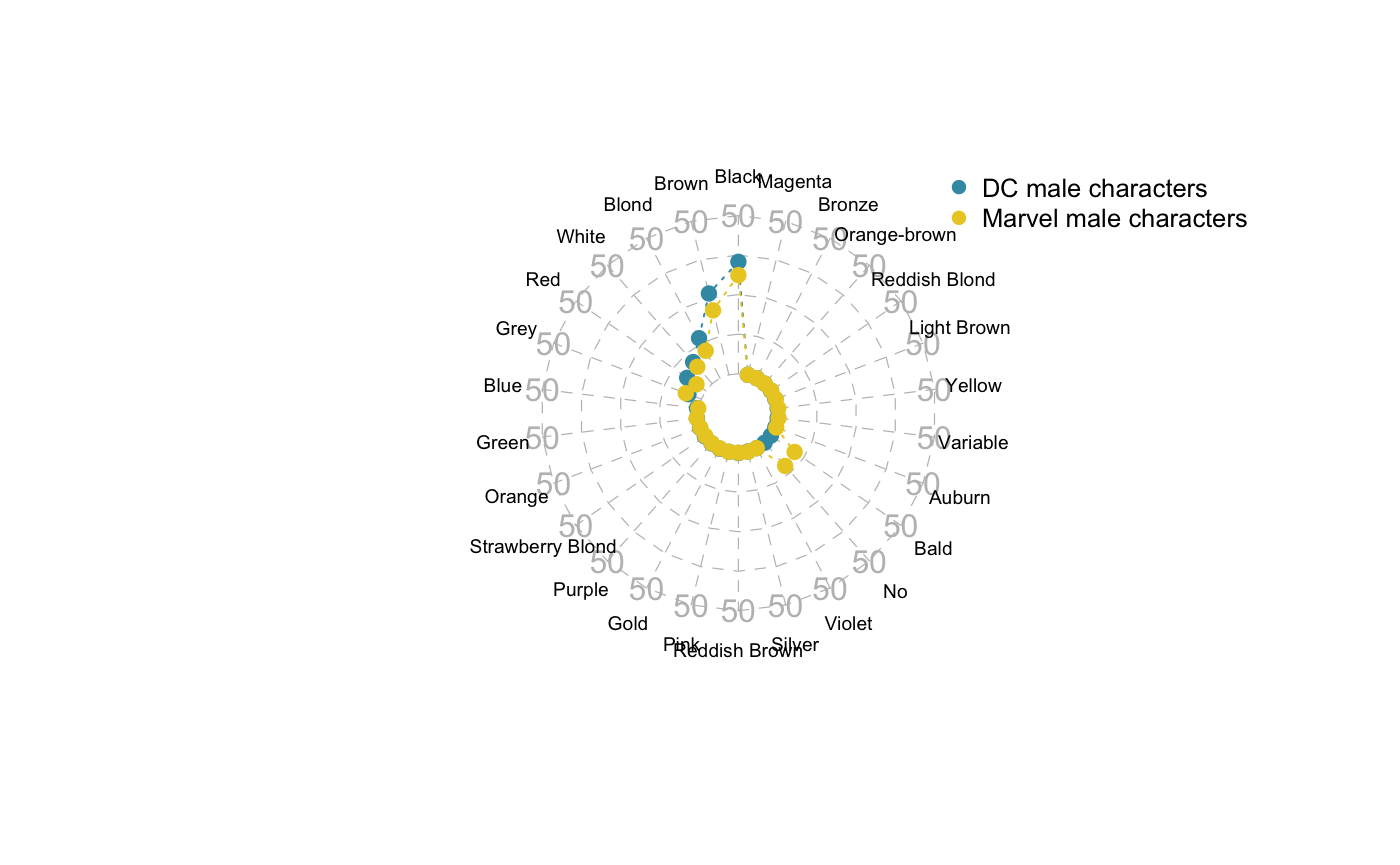
Characteristics per Gender, publisher

To represent the average characteristics, radarchart will be used.

Characteristics looked at are : id,align,eye,hair and alive.
the idea is to group the rows by these features and compute their mean
later by taking the higher percentage, we can deduce a profile representative of each publisher.

example: vs `Hair` feature

#function to aggregate data by (gender, feature, publisher)
aggregateFeature <- function(current_publisher, feature){
  #empty list to keep dataframe by (gender, feature)
  currentFeature <- list()
  if(current_publisher == 'Marvel'){
    gender_list <- gender_list_marvel
  } else {
    gender_list <- gender_list_dc
  }

  for(i in 1:length(gender_list)){
    currentFeature[[i]] <- comic_characters %>%
      filter(publisher == current_publisher ) %>%
      select(hair, sex) %>%
      na.omit() %>%
      group_by(hair) %>%
      filter(sex == gender_list[i]) %>%
      summarise(number = n()) %>%
      arrange(-number) %>%
      mutate(countT = sum(number)) %>%
      mutate(percentage = round(100*number/countT,1)) %>%
      select(hair, percentage, number)

    if(current_publisher == 'Marvel'){
      colnames(currentFeature[[i]])[2]<-'percentage_marvel'
    } else{
      colnames(currentFeature[[i]])[2]<-'percentage_dc'
    }

    if(feature == 'hair'){
      #strip 'hair' word for better display of the radarchart
      currentFeature[[i]]$hair <- sapply(currentFeature[[i]]$hair, function(x) gsub(' Hair','', x))}
  }

  names(currentFeature) <- gender_list
  return(currentFeature)
}

#outer join the 2 dataframes for (feature=Hair, gender=Male)
merged <- full_join(aggregateFeature('DC','hair')[[2]], aggregateFeature('Marvel','hair')[[2]], by='hair')
#set min/max percentages for the radarchart limits
min <- rep(0, length(merged$hair))
max <- rep(50, length(merged$hair))

maleHair <- data.frame(rbind(max,min,merged$percentage_dc,merged$percentage_marvel))
colnames(maleHair) <- merged$hair
row.names(maleHair) <- c('max','min','percentage_dc','percentage_marvel')
maleHair[is.na(maleHair)] <- 0

#cosmetics
radarchart(maleHair,                     #dataframe
           axistype=2,                   #axis type
           pcol=c("#3B9AB2", "#EBCC2A"), #color -Wes Anderson Sissou-
           plwd=1,                       #axis line width
           pty=19,                       #marker type
           plty=3,                       #line type
           cglcol="grey",                #axis line color
           cglty=2,                      #axis line type
           axislabcol="grey",            #Color of axis label
           cglwd=.6,                     #line type
           vlcex=.6,                     #font size label
           palcex=1.)                    #font size value
legend(x=1, y=1.3,                                               #position
       legend = c('DC male characters','Marvel male characters'),#labels
       bty="n",                                                  #no window
       pch=16,                                                   #marker type 
       text.col = "black",                                       #label colors 
       col=c("#3B9AB2","#EBCC2A"),                               #marker color
       cex=.8,                                                   #marker size 
       pt.cex=1)                                                 #font size

Popularity

By looking at the number of appearances for each characters, we can make a visualization (wordcloud) representing the most popular characters.

#remove NA from appearance column, keep only the name inside parentheses
marvel_appearances <- comic_characters %>%
  filter(publisher == 'Marvel') %>%
  select(name, appearances) %>% na.omit() %>%
  mutate(name = gsub(" *\\(.*?\\) *", "", name))
dc_appearances <- comic_characters %>%
  filter(publisher == 'DC') %>%
  select(name, appearances) %>% na.omit() %>%
  mutate(name = gsub(" *\\(.*?\\) *", "", name))

color_marvel <- colorRampPalette(c("#EBCC2A", "black"))
color_dc <- colorRampPalette(c("#3B9AB2", "black"))

op <- par(mar = c(1, 2, 2, 1), mfrow = c(1, 2))
wordcloud(dc_appearances$name, dc_appearances$appearances, min.freq = 100, colors = color_dc(10), scale = c(1.75, 0.2))
wordcloud(marvel_appearances$name, marvel_appearances$appearances, min.freq = 250, colors = color_marvel(10), scale = c(1.5, 0.2))

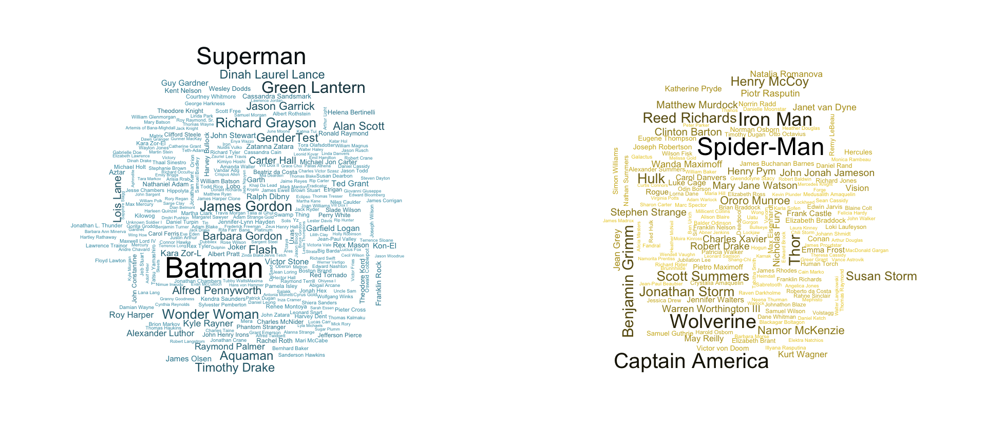
Batman(DC) and Spider-Man(Marvel) ends up being the characters with the most appearances.

Jonathan Bouchet

2020-08-11

Overview plots

Overview plots

Number of Characters vs. Time

Characteristics per Gender, publisher

example: vs `Hair` feature

Popularity

Gender in Comic Books

Jonathan Bouchet

2020-08-11

Overview plots

Overview plots

Number of Characters vs. Time

Characteristics per Gender, publisher

example: vs Hair feature

Popularity

example: vs `Hair` feature