Trump Twitter analysis using the tidyverse
Adam Spannbauer and Jennifer Chunn
2020-08-11
trump_twitter.RmdThis vignette is based on data collected for the 538 story entitled “The World’s Favorite Donald Trump Tweets” by Leah Libresco available here.
Load required packages to reproduce analysis.
library(fivethirtyeight)
library(ggplot2)
library(dplyr)
library(readr)
library(tidytext)
library(textdata)
library(stringr)
library(lubridate)
library(knitr)
library(hunspell)
# Turn off scientific notation
options(scipen = 99)
Check date range of tweets
## check out structure and date range ------------------------------------------------
(minDate <- min(date(trump_twitter$created_at)))
## [1] "2015-08-01"## [1] "2016-08-16"Create vectorised stemming function using hunspell
my_hunspell_stem <- function(token) {
  stem_token <- hunspell_stem(token)[[1]]
  if (length(stem_token) == 0) return(token) else return(stem_token[1])
}
vec_hunspell_stem <- Vectorize(my_hunspell_stem, "token")
Clean text by tokenizing & removing urls/stopwords
We first remove URLs and stopwords as specified in the tidytext library. Stopwords are common words in English. We also do spellchecking using hunspell.
trump_tokens <- trump_twitter %>%
  mutate(text = str_replace_all(text,
                                pattern=regex("(www|https?[^\\s]+)"),
                                replacement = "")) %>% #rm urls
  mutate(text = str_replace_all(text,
                                pattern = "[[:digit:]]",
                                replacement = "")) %>%
  unnest_tokens(tokens, text) %>% #tokenize
  mutate(tokens = vec_hunspell_stem(tokens)) %>%
  filter(!(tokens %in% stop_words$word)) #rm stopwords
Sentiment analysis
To measure the sentiment of tweets, we used the AFINN lexicon for each (non-stop) word in a tweet. The score runs between -5 and 5. We then sum the scores for each word across all words in one tweet to get a total tweet sentiment score.
afinn_sentiment <- system.file("extdata", "afinn.csv", package = "fivethirtyeight") %>%
  read_csv()
## Parsed with column specification:
## cols(
##   word = col_character(),
##   value = col_double()
## )
trump_sentiment <- trump_tokens %>% inner_join(afinn_sentiment, by=c("tokens"="word")) trump_full_text_sent <- trump_sentiment %>% group_by(id) %>% summarise(score = sum(value, na.rm=TRUE)) %>% ungroup() %>% right_join(trump_twitter, by="id") %>% mutate(score_factor = ifelse(is.na(score), "Missing score", ifelse(score < 0, "-.Negative", ifelse(score == 0, "0", "+.Pos"))))
## `summarise()` ungrouping output (override with `.groups` argument)Distribution of sentiment scores
trump_full_text_sent %>%
  count(score_factor) %>% mutate(prop = prop.table(n))
## # A tibble: 4 x 3
## score_factor n prop
## <chr> <int> <dbl>
## 1 -.Negative 59 0.132
## 2 +.Pos 173 0.386
## 3 0 8 0.0179
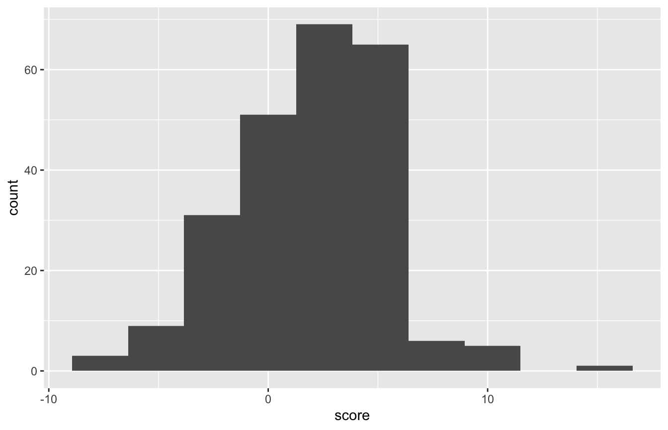
## 4 Missing score 208 0.46446.4% of tweets did not have sentiment scores. 15.4% were net negative and 36.6% were net positive.
ggplot(data=trump_full_text_sent, aes(score)) +
  geom_histogram(bins = 10)
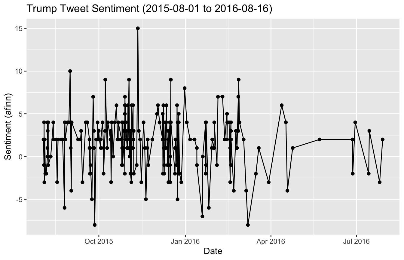
plot sentiment over time
sentOverTimeGraph <- ggplot(data=filter(trump_full_text_sent,!is.na(score)), aes(x=created_at, y=score)) +
  geom_line() +
  geom_point() +
  xlab("Date") +
  ylab("Sentiment (afinn)") +
  ggtitle(paste0("Trump Tweet Sentiment (",minDate," to ",maxDate,")"))
sentOverTimeGraph
Examine top 5 most positive tweets
most_pos_trump <- trump_full_text_sent %>%
  arrange(desc(score)) %>%
  head(n=5) %>%
  .[["text"]]

kable(most_pos_trump, format="html")
| x |
|---|
| Loved doing the debate…won Drudge and all on-line polls! Amazing evening, moderators did an outstanding job. |
| Loved being with my many friends in Tennessee. The crowd and enthusiasm was fantastic. I won the straw poll big! |
| Just found out I won the Rockingham County Republican Booth Straw Poll at the Deerfield Fair in New Hampshire this past weekend. 39% —Wow! |
| Thank you @JoeTrippi for the nice, and true, words on #Media Buzz with terrific Howie Kurtz. Leading New Hampshire 30 to 12. @FoxNews |
| Thank you, so many people have given me credit for winning the debate last night. All polls agree. It was fun and interesting! |
Examine top 5 most negative tweets
most_neg_trump <- trump_full_text_sent %>%
  arrange(score) %>%
  head(n=5) %>%
  .[["text"]]
kable(most_neg_trump, format = "html")
| x |
|---|
| Marco Rubio is a member of the Gang Of Eight or, very weak on stopping illegal immigration. Only changed when poll numbers crashed. |
| Failed presidential candidate Lindsey Graham should respect me. I destroyed his run, brought him from 7% to 0% when he got out. Now nasty! |
| Ted Cruz is falling in the polls. He is nervous. People are worried about his place of birth and his failure to report his loans from banks! |
| .@GovernorPataki did a terrible job as Governor of New York. If he ran again, he would have lost in a landslide. He and Graham ZERO in polls |
| Ted Cruz is a nervous wreck. He is making reckless charges not caring for the truth! His poll #’s are way down! |
When is trumps favorite time to tweet?
Total number of tweets and average sentiment (when available) by hour of the day, day of the week, and month
trump_tweet_times <- trump_full_text_sent %>%
  mutate(weekday = wday(created_at, label=TRUE),
         month   = month(created_at, label=TRUE),
         hour    = hour(created_at),
         month_over_time = round_date(created_at,"month"))

plotSentByTime <- function(trump_tweet_times, timeGroupVar) {
  timeVar <- substitute(timeGroupVar)
  timeVarLabel <- str_to_title(timeVar)

  trump_tweet_time_sent <- trump_tweet_times %>%
    rename(timeGroup = !! timeVar) %>%
    group_by(timeGroup) %>%
    summarise(score = mean(score, na.rm=TRUE), Count = n()) %>%
    ungroup()

  ggplot(trump_tweet_time_sent, aes(x=timeGroup, y=Count, fill = score)) +
    geom_bar(stat="identity") +
    xlab(timeVarLabel) +
    ggtitle(paste("Trump Tweet Count & Sentiment by", timeVarLabel))
}
plotSentByTime(trump_tweet_times, "hour")
## `summarise()` ungrouping output (override with `.groups` argument)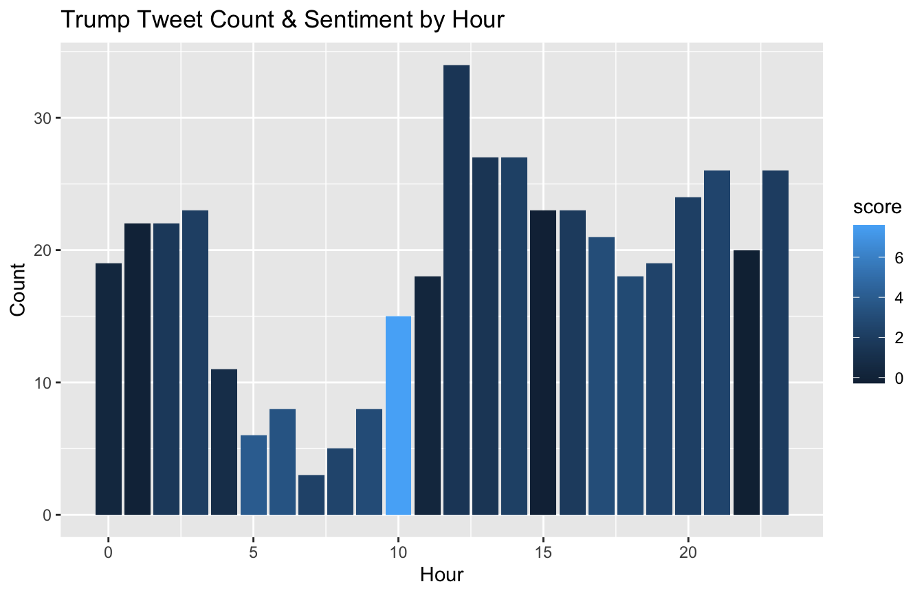
- Trump tweets the least between 4 and 10 am.
- Trump’s tweets are most positive during the 10am hour.
plotSentByTime(trump_tweet_times, "weekday")
## `summarise()` ungrouping output (override with `.groups` argument)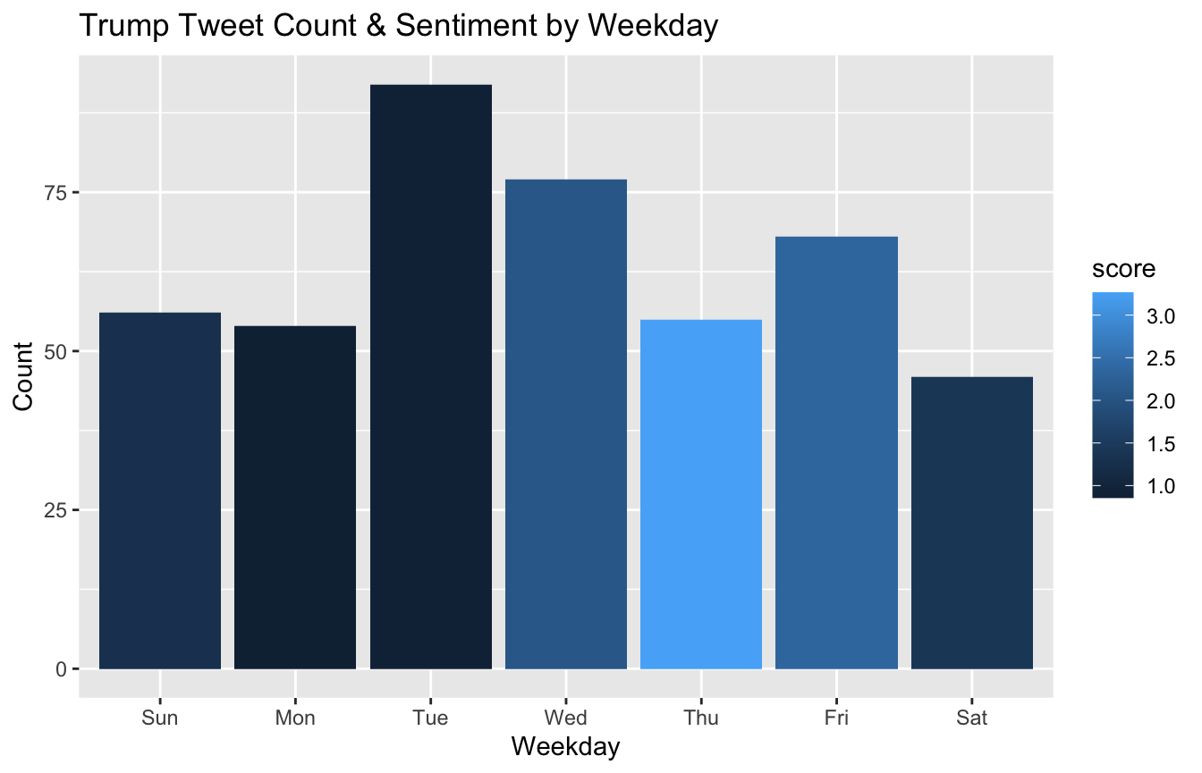
- Trump tweeted the most on Tuesday and Wednesday
- Trump was most positive in the second part of the work week (Wed, Thurs, Fri)
plotSentByTime(trump_tweet_times, "month_over_time")
## `summarise()` ungrouping output (override with `.groups` argument)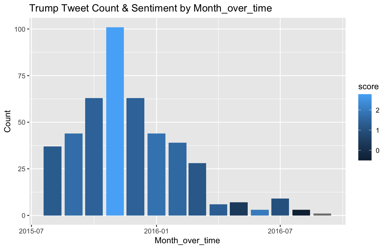
- In this dataset, the number of tweets decreased after November 2015 and drastically dropped off after March 2016. It is unclear if this is a result of actual decrease in tweeting frequency or a result of the data collection process.